CUDA Matrix-multiplication
My Work
- Neural network (NN) trained for number recognition
- Writing feedforward and backpropogation kernels in CUDA
- GPU implementation of NN logic using CUDA kernels
- Optimization of GPU kernels
- Profiling using NSight Compute
You can check out a blogpost I made on this project using the following link: building a matrix-multiplication kernel from scratch using CUDA and applying it to neural networks. This project was made in custom engine, where the engine is C++ and the CUDA kernels use hlsl for the compute shaders.
Performance Of Matrix Multiplication On The GPU
Matrix multiplication is the core of neural networks, this is how the input you use traverses the NN until it reaches the end and is returned. The multiplication of matrices on the GPU has been optimized a lot and there are many sources online that explain different optimizations. The main source I used was: OpenCL SGEMM tuning for Kepler. It explains the concepts of the optimizations in an easy to understand and visual way. Eventhough it uses OpenCL, it is easily translated to CUDA. We will go over a couple of optimization steps, that I have implemented in my matrix multiplication kernel. If you are unfamiliar with how the GPU works, then I recommend checking out the article I wrote, it contains a short introduction into how the GPU works.
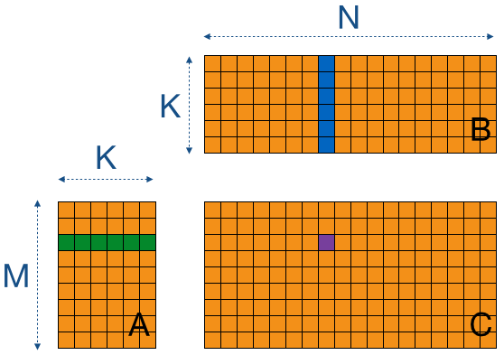
Matrix multiplication is taking the dot product between a row from matrix A and a column from matrix B to get the value of the element of the output matrix C in the corresponding row and column. In the adjacent image there is a visualization used in the tutorial that shows this concept. Implementing this on the GPU is easy enough, but it is not very fast. The main cause for this is the amount of global memory loads per thread.
We can minimize global memory reads by using shared memory, we read sub-blocks of matrices A and B into shared memory and execute the dot product calculation for these smaller sub-blocks (tiles). We can use these tiles to step over the entirety of matrices A and B. You can set the value of an element in the tile to 0, if the tile size does not allign perfectly with the rows and culumns to account for overshoot.
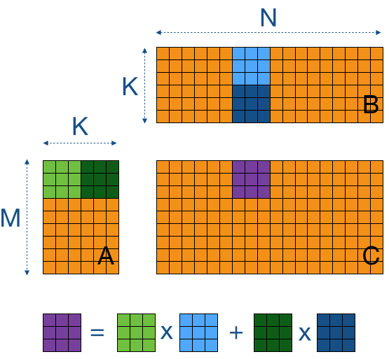
The next optimization step is increasing the workload per thread. While tile based matrix multiplication is already an improvement to basic matrix multiplication, it is not utilizing the GPU to its fullest. The following step makes better use of the GPU, by increasing the arithmetic intensity (more instructions per read from memory) for each thread and reducing the number of threads.
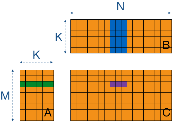
In the image below, the highlighted row from matrix A has to be used for each column of matrix B, to calculate the values for each element in that row in matrix C. To minimize the memory reads from matrix A, it is possible to read the row from matrix A once and use it for multiple columns of matrix B before reading another row from matrix A. Only 3 columns are used at a time in the image below, once these three columns have been used for the dot product computation, three new columns will be stored in shared memory.
For simplicity the example does not consider the tiling optimization done before, but the same concept of this step can be applied to the tiles used in tile based GEMM. Instead of storing an entire row and columns, you read parts of them depending on the tile size.
Matrix Multiplication In Neural Networks
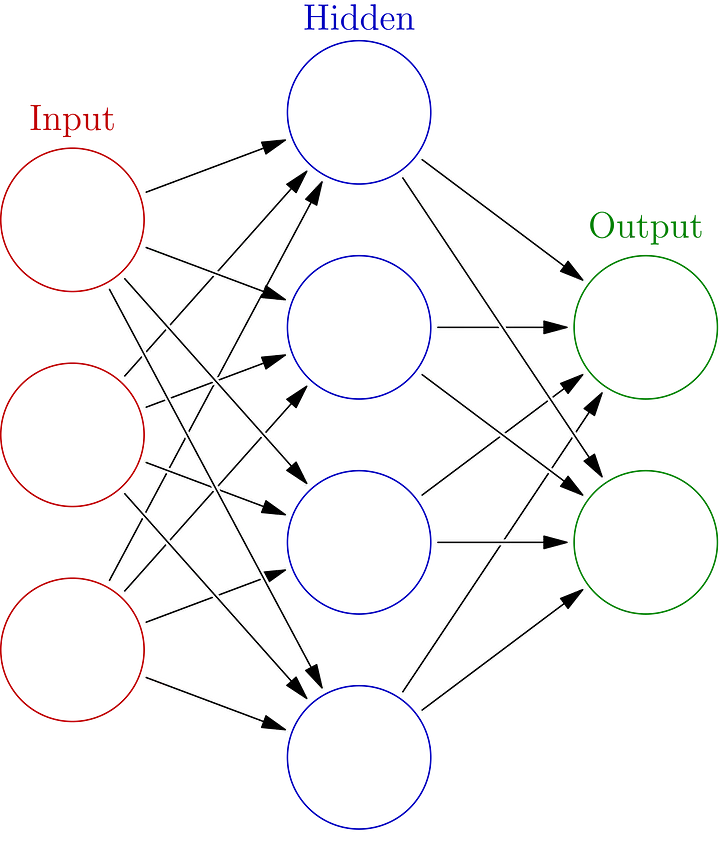
Now that we have a basic understanding of the GPU and how to utilize the GPU for matrix multiplication, we can take a look at how this applies to NNs. The architecture of a multi layer peceptron (NN) is given in the image below. Some input goes in, passes through the NN and gives some output. Passing through the NN (forward propogation), is something that happens layer after layer, starting from the input layer, continuing through all the hidden layers and finally finishes with the output layer. The computation that happens to go from one layer to the next is matrix multiplication and the values of all neurons (nodes in a layer) are independent from the other neurons in the same layer. So they can be done in parallel and the GPU is perfect for this.
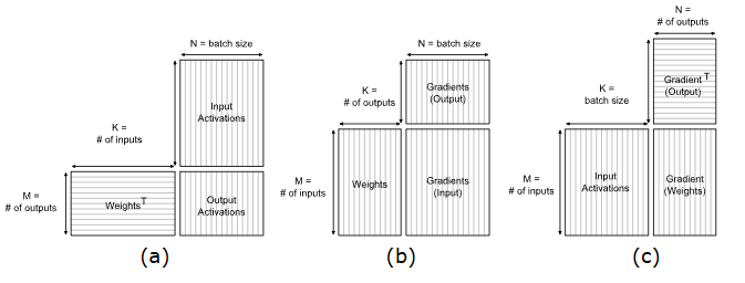
Using this method to move from layer to layer is the state-of-the-art method used by PyTorch, Caffe and Tensorflow according to the Nvidia documentation (Fully-connected layer Nvidia docs). The adjacent image shows the matrices used as inputs to determine the output for different computations of the NN. Forward propogation (a) is used to test the GEMM kernel I have made, but the other computations are important for backpropogation (training of a NN).
CPU vs GPU
The main reason to use the GPU for NN computations is because it is faster than the CPU, if implemented correctly. So it is important to compare the GPU implementation to a CPU implementation I had made before. To perform this comparison I used a batch size of 256 and network size of:
- Input layer: 784
- Hidden layer: 100 (relu)
- Hidden layer: 100 (relu)
- Output layer: 10 (softmax)
| Version | Duration (ms) |
|---|---|
| CPU | 22 |
| GPU (tile-based GEMM) | 43.22 |
| GPU (more work per thread) | 21.25 |
| GPU (more WPT + improved memory access pattern) | 6.5 |
The tile based matrix multiplication implementation I had made was about 2 times slower than the CPU version. This was mostly because of a poor utilization of the GPU. By profiling the kernel (with Nsight Compute) I was able to determine the bottlenecks and improve the performance. Improving the matrix multiplication made the kernel about the same speed as the CPU version, but there were still some big bottlenecks regarding memory access patterns. A lot of time was spent idle on the threads, waiting for data. The data I stored in shared memory was uncoalesced, meaning I was accessing a value of the stored matrix, then had to jump a couple of bytes in memory to find the next value. I coalesced the data in memory by changing the memory access pattern. Now when accessing data in memory, I can read a value and the next value I need is adjacent to the read value (no more jumping of bytes to find the correct value). The resulting kernel is 70.45% faster than the CPU version, which is a significant performance improvement.
Demo
I made a small demo using the matrix multiplication kernel for forward propogation of a trained NN, to demonstrate the kernel in action. The user can draw a digit in the ImGui window and the NN tries to classify the drawn digit in real time.